HOW A JUNCTION IS CALCULATED
Every step of a real calculation, from the CAD drawing to the ψ-value, shown on one detail — the timber-frame box lintel published as a worked example. The figures on this page are read from that example's own generated output, not written by hand, so each step can be traced to the run that produced it.
Six steps. The drawing is never redrawn, no value is estimated where it can be solved, and the finished report is published in full at the end.
- Step 1
Start from the CAD drawing you already have
The detail is drawn in CAD as an ordinary cross-section and exported as a DXF. Nothing is redrawn inside Psiclops. On import the file is parsed into closed regions — the areas that will become materials — and the parser reports exactly what it found, including anything it could not close. That report is the first thing to check, because a drawing that does not close cleanly is the one real failure mode of a CAD-led route, and it is caught here rather than surfacing later as a wrong answer.
Source fileLintel-Sketcha.dxfClosed regions found13Dangling line ends0Cuts needed0Warnings0Errors0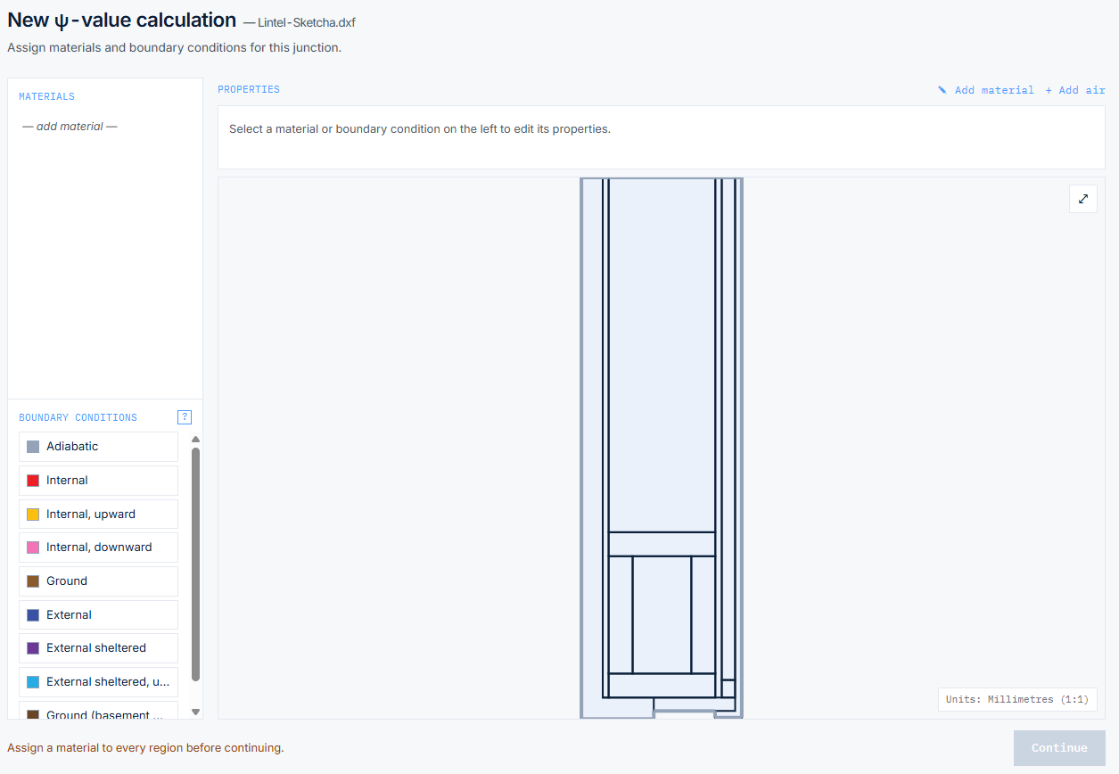
The drawing as imported. Every closed region has been found and none can be calculated yet — Psiclops will not continue until each one has a material. - Step 2
Assign materials, air and boundary conditions
One screen, because these are one job. Each closed region takes a material — from the library or entered directly, each carrying its own provenance so the report can cite where the conductivity came from — and each exposed edge is tagged internal, external or adiabatic. Air is assigned here too, as a region in its own right rather than a gap. Two things are then resolved for you. An air space has no conductivity to look up: its resistance follows from its thickness, the direction of heat flow, whether it is a cavity or a void sealed inside the construction, and the emissivity of the surfaces facing it, resolved by BS EN ISO 6946 Annex B and BR 497 §2.4. And an internal edge that turns out to be near-horizontal is a ceiling or a floor rather than a wall, so it takes the surface resistance for that direction of heat flow — the lintel soffit here is exactly that case. One region is not a plain material at all: the insulated I-joist bay is a whole 2D assembly, modelled separately and referenced here, its equivalent conductivity solved from that model rather than estimated.
Boundary edges13Section orientationverticalAir space25 mm cavity horizontalResolved resistance0.183 m²K/WEquivalent conductivity0.1366 W/(m·K)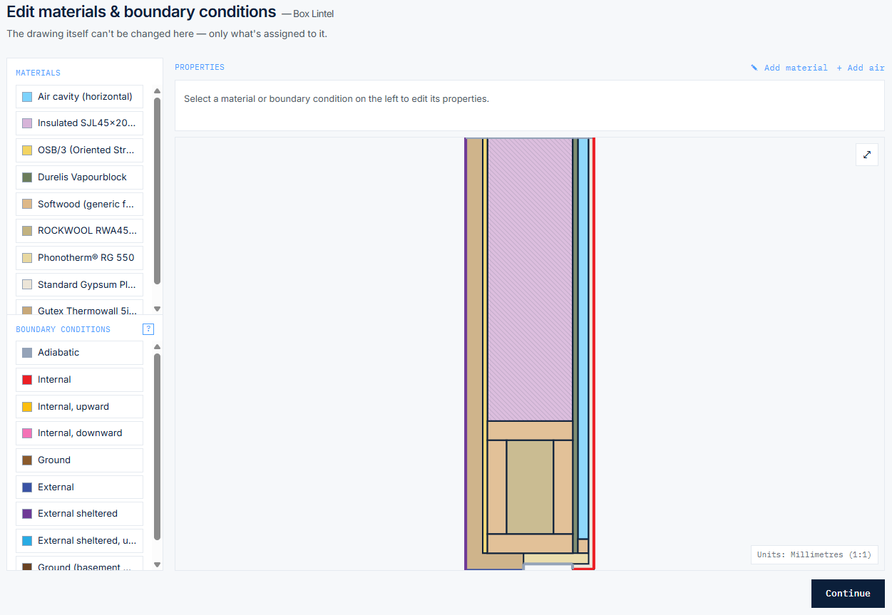
Every region assigned and every exposed edge tagged. The air cavity appears in the material list alongside the solids, and the I-joist bay is the referenced assembly. - Step 3
Mesh, and keep refining until the answer stops moving
The section is meshed and solved by finite element analysis. A single solve is not enough: BR 497 §2.6 requires the mesh to be refined and the problem re-solved until the answer stops changing — the heat flow within 1% and the temperature factor within 0.005 between successive refinements. The figures below are that test as it actually ran: the heat flow at each level, and the change between them. The mesh was not chosen in advance; it is where the criterion was met.
Elements at convergence6,454Nodes3,341Refinement levels solved2Heat flow by level3.8227 W/m → 3.8154 W/mChange at final level0.19%BR 497 §2.6 tolerance1%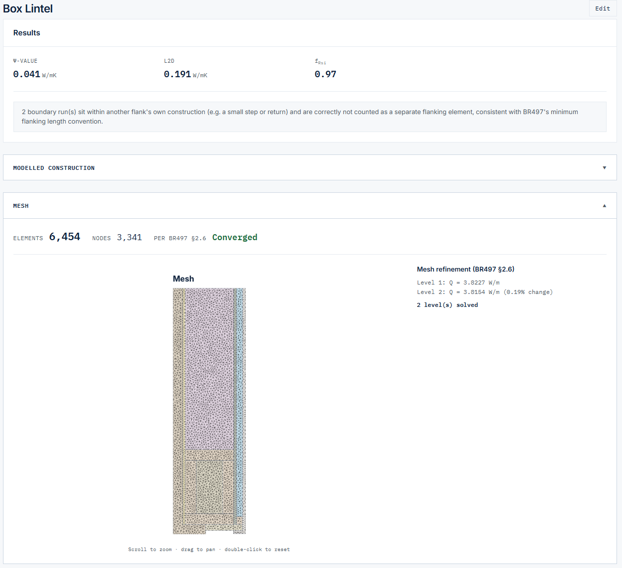
The mesh the convergence test settled on, with the heat flow at each refinement level shown beside it — the same figures recorded above. - Step 4
Read the result — and the evidence behind it
The ψ-value and the temperature factor come out of the solved field, each shown with the figure it is judged against, and with the arithmetic in view rather than summarised. This is where the headline comparison comes from: SAP Table K1 assigns this junction type a default ψ-value to be used when no bespoke calculation exists, and the calculated value is what replaces it.
SAP Table K1 default ψ1.000 W/(m·K)Calculated ψ0.041 W/(m·K)Temperature factor0.966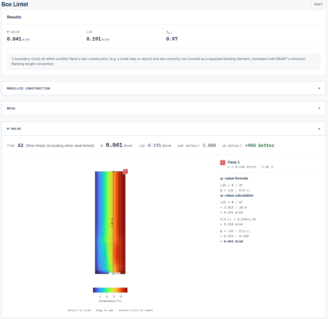
The result, with the arithmetic shown rather than summarised: the flanking element removed from L2D to leave ψ, and the SAP default it is compared against. - Step 5
Check the condensation risk
The same solved field answers a second question: whether moisture will condense inside the construction. This step appears only when every material carries vapour data — a resistivity (μ) or an Sd value — because without it there is nothing to compare, and Psiclops says the check was skipped and why rather than reporting a pass it cannot support. Given that data, it compares vapour pressure against saturation pressure across the whole 2D cross-section, rather than walking a single ordered inside-to-outside layer path as the classic 1D Glaser method does — which is why it can find a worst point at an interface a layer-walk would never have looked at. The verdict comes with its margin, its location and the interface it was found at, so a narrow pass reads as a narrow pass. A margin this size is worth taking further: it is a steady-state result under design conditions, and air leakage, local cold bridging or a harder winter than those conditions assume can all erode it, none of which this check can see. Where that matters, the annual condensation check — run through Psiclops Assist — models the full year rather than a single design point.
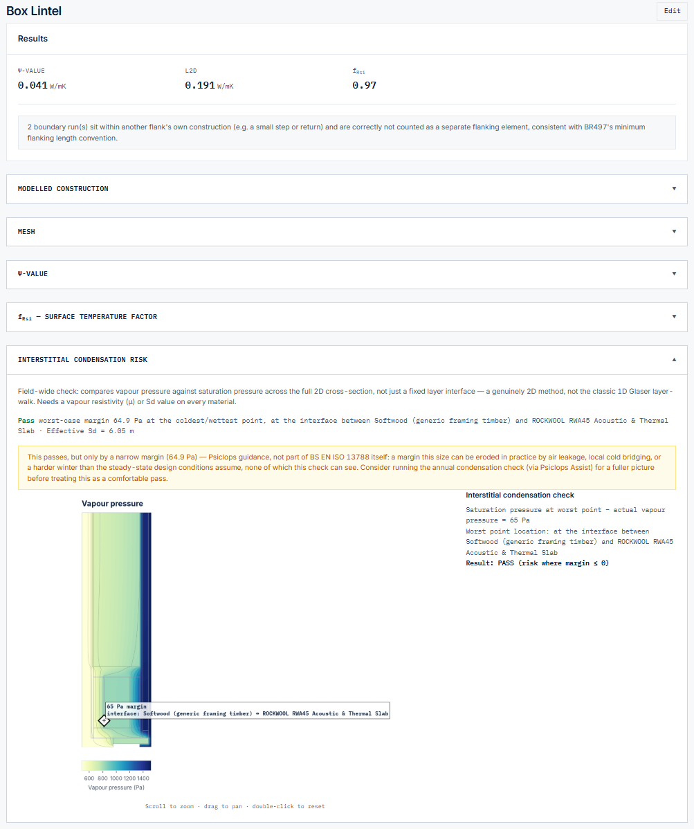
A pass, with the margin stated and flagged as a narrow one — and the vapour pressure field showing where the worst point sits, at the softwood-to-mineral-wool interface. - Step 6
Take it to the full year with Psiclops Assist
A steady-state pass is a single design point. Psiclops Assist answers the harder question: what happens across a whole year. It opens with the junction already loaded — its summary, its material schedule, its drawing — and runs the annual interstitial condensation analysis node by node across the entire 2D cross-section, under EN ISO 13788's annual-cycle method, rather than at fixed 1D layer interfaces. It runs against a real climate normal for the project's own coordinates, which is the compliance basis, and runs the standard's own fixed UK-wide reference climate alongside it for comparison, so a result that depends on which climate was assumed is visible as exactly that. For this lintel the peak accumulated moisture was zero and the construction cleared the cycle outright. From there the junction stays in view: you can ask questions about it and have material substitutions proposed against it, without rebuilding anything. Assist is included with Pro.
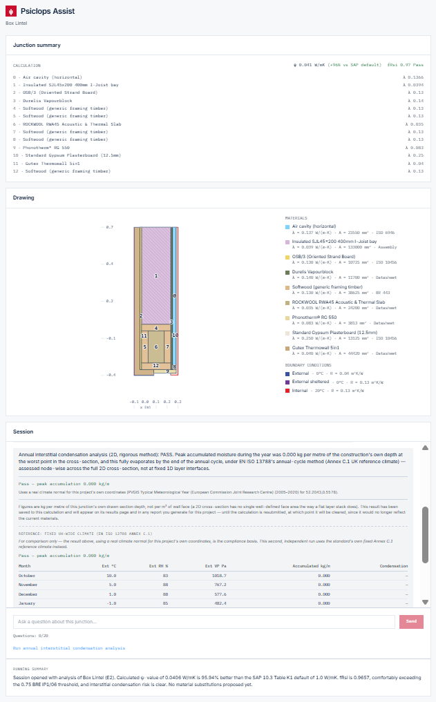
The annual analysis, month by month, beside the junction it belongs to — with the climate it was run against named rather than assumed.
The finished report
The complete report for this detail — the referenced I-joist bay assembly, the junction, the ψ-value summary and the temperature factor — is published in full, rendered by the same components a real project report uses. Steps 5 and 6 above are shown from the app rather than from this report; for a published condensation analysis, see the BR 497 worked example.
Read the full worked example →Nothing on this page was calculated live. It describes a calculation that was run once, offline, by Psiclops's own engine, and whose output is published unchanged. Try your own junction for free →